How To Draw Phase Portrait

Stage Portraits of Linear Systems

Consider a $2 \times 2$ linear homogeneous organisation ${\bf x}' = A {\bf x}$ . We think of this equally describing the motility of a indicate in the $xy$ plane (which in this context is called the stage plane), with the contained variable $t$ as fourth dimension. The path travelled by the point in a solution is called a trajectory of the system. A picture of the trajectories is called a phase portrait of the system. In the blithe version of this folio, you tin can meet the moving points likewise as the trajectories. Only on paper, the best nosotros can practice is to apply arrows to signal the management of move.

In this section we study the qualitative features of the stage portraits, obtaining a classification of the different possibilities that tin can arise. One reason that this is of import is because, as we will see shortly, it will be very useful in the study of nonlinear systems. The nomenclature volition not exist quite complete, because we'll leave out the cases where 0 is an eigenvalue of $A$ .

The first step in the classification is to discover the characteristic polynomial, $\mbox{det}\,(A - r I)$ , which will be a quadratic: we write it equally $r^2 + p r + q$ where $p$ and $q$ are real numbers (assuming equally usual that our matrix $A$ has real entries). The classification will depend mainly on $p$ and $q$ , and we brand a nautical chart of the possibilities in the $pq$ plane.

Now we look at the discriminant of this quadratic, $p^2 - 4 q$ . The sign of this determines what type of eigenvalues our matrix has:

$Image stabil.gif$

Each of these cases has subcases, depending on the signs (or in the complex case, the sign of the real role) of the eigenvalues. Notation that $q$ is the product of the eigenvalues (since $r^2 + p r + q = (r - r_1)(r - r_2)$ ), so for $p^2 - 4 q > 0$ the sign of $q$ determines whether the eigenvalues accept the same sign or opposite sign. Nosotros will ignore the possibility of $q=0$ , equally that would mean 0 is an eigenvalue.

The sum of the eigenvalues is $-p$ , and then if they have the same sign this is opposite to the sign of $p$ . If the eigenvalues are complex, their real part is $-p/2$ .

Another of import tool for sketching the phase portrait is the following: an eigenvector ${\bf u}$ for a existent eigenvalue $r$ corresponds to a solution $\displaystyle {\bf x}= {\rm e}^{r t} {\bf u}$ that is always on the ray from the origin in the direction of the eigenvector ${\bf u}$ . The solution $\displaystyle {\bf x}= - {\rm e}^{rt} {\bf u}$ is on the ray in the opposite direction. If $r > 0$ the motion is outward, while if $r < 0$ it is inwards. As $t \to -\infty$ (if $r > 0$ ) or $+\infty$ (if $r < 0$ ), these trajectories arroyo the origin, while as $t \to +\infty$ (if $r > 0$ ) or $-\infty$ (if $r < 0$ ) they go off to $\infty$ . For circuitous eigenvalues, on the other hand, the eigenvector is not so useful.

In addition to a nomenclature on the basis of what the curves expect like, nosotros will want to talk over the stability of the origin as an equilibrium point.

Hither, and so, is the classification of the phase portraits of $2 \times 2$ linear systems.

If $p^2 - 4 q > 0$ , $q > 0$ and $p > 0$ , we have 2 negative eigenvalues. There are straight-line trajectories respective to the eigenvectors. The other trajectories are curves, which come in to the origin tangent to the ``slow'' eigenvector (corresponding to the eigenvalue that is closer to 0), and as they go off to $\infty$ approach the direction of the ``fast'' eigenvector.
This case is called a node. Information technology is an attractor.

Here is the picture for the matrix 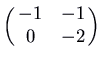$\displaystyle \pmatrix{-1 & -1\cr 0 & -2\cr}$ , which has characteristic polynomial $r^2 + 3 r + 2$ . The eigenvalues are $-1$ (slow) and $-2$ (fast), respective to eigenvectors $\displaystyle \pmatrix{1\cr 0\cr}$ and $\displaystyle \pmatrix{1\cr 1\cr}$ respectively.

$Image anode.gif$
If $p^2 - 4 q > 0$ , $q > 0$ and $p < 0$ , nosotros have 2 positive eigenvalues. The picture is the same as in the previous instance, except with the arrows reversed (going outward instead of in). Once more the curved trajectories come in to the origin tangent to the ``slow'' eigenvector (corresponding to the eigenvalue that is closer to 0), and every bit they become off to $\infty$ arroyo the direction of the ``fast'' eigenvector. This is too a node, simply it is unstable. Here is the pic for the matrix $\displaystyle \pmatrix{1 & 1\cr 0 & 2\cr}$ , which has characteristic polynomial $r^2 - 3 r + 2$ . The eigenvalues are $1$ (slow) and $2$ (fast), respective to eigenvectors $\displaystyle \pmatrix{1\cr 0\cr}$ and $\displaystyle \pmatrix{1\cr 1\cr}$ respectively. Note that the flick is exactly the aforementioned equally what we had for the attractor node, except that the direction of time is reversed (the animation is run backwards).
$Image node.gif$
If $p^2 - 4 q > 0$ and $q < 0$ , we have 1 positive and one negative eigenvalue. Again there are directly-line trajectories corresponding to the eigenvectors, with the motion outwards for the positive eigenvalue and inwards for the negative eigenvalue. These are the only trajectories that approach the origin (in the limit every bit $t \to -\infty$ for the positive and $t \to +\infty$ for the negative eigenvalue). The other trajectories are curves that come in from $\infty$ asymptotic to a straight-line trajectory for the negative eigenvalue, and go back out to $\infty$ asymptotic to a direct-line trajectory for the positive eigenvalue.
This is called a saddle. Information technology is unstable. Note that if yous start on the straight line in the direction of the negative eigenvalue yous do approach the equilibrium signal as $t \to \infty$ , just if you start off this line (even very slightly) yous finish up going off to $\infty$ .

Here is the picture for the matrix $\displaystyle \pmatrix{1 & -2\cr 0 & -1\cr}$ , which has characteristic polynomial $r^2 - 1$ . The eigenvalues are $1$ and $-1$ , corresponding to eigenvectors $\displaystyle \pmatrix{1\cr 0\cr}$ and $\displaystyle \pmatrix{1\cr 1\cr}$ respectively.

$Image saddle.gif$
If , we take only 1 eigenvalue (a double eigenvalue). There are two cases here, depending on whether or non there are ii linearly independent eigenvectors for this eigenvalue.
1. If there are two linearly independent eigenvectors, every nonzero vector is an eigenvector. Therefore we accept directly-line trajectories in all directions. The motion is e'er inward if the eigenvalue is negative (which ways $p > 0$ ), or outwards if the eigenvalue is positive ( $p < 0$ ). This is chosen a singular node. It is an attractor if $p > 0$ and unstable if $p < 0$ .
  Here is the picture for the matrix $\displaystyle I = \pmatrix{1 & 0\cr 0 & 1\cr}$ , which has characteristic polynomial $r^2 - 2 r + 1$ and eigenvalue $1$ . It is unstable. For the matrix $-I$ we would accept an attractor: the aforementioned motion picture except with fourth dimension reversed.
  
  $Image snode.gif$
2. If there is only one linearly independent eigenvector, there is but one straight line. The other trajectories are curves, which come up in to the origin tangent to the straight line trajectory and curve around to the opposite direction. Trajectories on opposite sides of the direct line class an ``South'' shape. The way to tell whether it is a forrard S or backwards S is to look at the direction of the velocity vector ${\bf x}'$ at some bespeak off the straight line.
  This is chosen a degenerate node. Once more, it is an attractor if $p > 0$ and unstable if $p < 0$ .
  
  Hither is the motion picture for the matrix $\displaystyle A = \pmatrix{2 & 1\cr -1 & 0\cr}$ , which has characteristic polynomial $r^2 - 2 r + 1$ , eigenvalue 1 and eigenvector $\displaystyle \pmatrix{1 \cr -1\cr}$ . It is unstable. Annotation that the trajectories in a higher place the directly line $y=-x$ are come up out of the origin heading to the left along that line, and those beneath the line come out heading to the right. Thus the S is frontward. To check this, yous could summate the velocity vector at, for case, $\displaystyle \pmatrix{0\cr 1\cr}$ , which is $\displaystyle A \pmatrix{0\cr 1\cr} = \pmatrix{ 1\cr 0\cr}$ . Since that points to the right, information technology's easy to see the Due south must exist forwards.
  
  $Image dnode.gif$
If $p^2 - 4 q < 0$ and $p \ne 0$ , we have complex eigenvalues $-p/2 \pm i \mu$ . The solutions are of the form $\displaystyle {\rm e}^{-pt/2}$ times some combinations of $\sin \mu t$ and $\cos \mu t$ . The picture is a screw, also known equally a focus. It is an attractor if $p > 0$ , as the factor $\displaystyle {\rm e}^{-pt/2}$ makes all solutions approach the origin as $t \to \infty$ , and unstable if $p < 0$ , as in that case the gene $\displaystyle {\rm e}^{-pt/2}$ makes all solutions (except the one starting at the equilibrium point itself) go off to $\infty$ as $t \to \infty$ . Nosotros can calculate a velocity vector to cheque if the motion is clockwise or counterclockwise.
Here is the pic for the matrix $\displaystyle \pmatrix{3 & 5\cr -8 & -1\cr}$ , which has characteristic polynomial $r^2 -2 r + 37$ and eigenvalues $1 \pm 6 i$ . It is unstable. To check that the motility is clockwise, y'all could note that the velocity vector at $\displaystyle \pmatrix{0\cr 1\cr}$ is $\displaystyle \pmatrix{5 \cr -1\cr}$ , which is to the right.
Finally, if $p^two - iv q < 0$ and $p = 0$ , we accept pure imaginary eigenvalues $\pm \sqrt{q} i$ . The solutions involve combinations of $\sin(\sqrt{q} t)$ and $\cos (\sqrt{q} t)$ . These are all periodic, with catamenia $2\pi/\sqrt{q}$ . The trajectories turn out to be ellipses centred at the origin. The picture is known as a centre. Since a solution that starts about the origin just goes around and around the aforementioned ellipse, never getting any closer to or farther from the equilibrium than the closest and uttermost points on the ellipse, this equilibrium is stable but non an attractor. Again nosotros can calculate a velocity vector to run across whether the motion is clockwise or counterclockwise.
Here is the picture for the matrix $\displaystyle \pmatrix{2 & 5\cr -8 & -2\cr}$ , which has characteristic polynomial $r^2 + 36$ and eigenvalues $\pm 6 i$ . Again you can check that the motion is clockwise by noting that the velocity vector at $\displaystyle \pmatrix{0\cr 1\cr}$ is $\displaystyle \pmatrix{5\cr -2\cr}$ , which is to the right.

$Image centre.gif$